On April 14, 2025, OpenAI released GPT-4.1 — a model touted as the new state-of-the-art, outperforming GPT-4o on all major benchmarks.
As always, I like to evaluate new LLMs on simple tasks like text classification and summarization to see how they compare with current leading models.
In this article, I will share the results I obtained for multi-class and multi-label text classification and text summarization using the OpenAI GPT-4.1 model. So, without further ado, let's begin.
Importing and Installing Required Libraries
The script below installs the Python libraries you need to run codes in this article.
!pip install openai
!pip install rouge-score
!pip install --upgrade openpyxl
!pip install pandas openpyxl
The following script imports the required libraries and modules into our Python application.
import pandas as pd
import matplotlib.pyplot as plt
import seaborn as sns
from itertools import combinations
from collections import Counter
from sklearn.metrics import hamming_loss, accuracy_score
from rouge_score import rouge_scorer
from openai import OpenAI

from google.colab import userdata
OPENAI_API_KEY = userdata.get('OPENAI_API_KEY')
Finally, we create the OpenAI client object we will use to call the OpenAI API. To access the API, you will need the OpenAI API key.
client = OpenAI(api_key = OPENAI_API_KEY)Text Summarization with GPT-4.1
We will first summarize articles in the News Article Summary dataset.
The following script imports the dataset into your application and displays its first five rows.
# https://github.com/reddzzz/DataScience_FP/blob/main/dataset.xlsx


dataset = pd.read_excel(r"/content/summary_dataset.xlsx")
print(dataset.shape)
dataset.head()
Output:
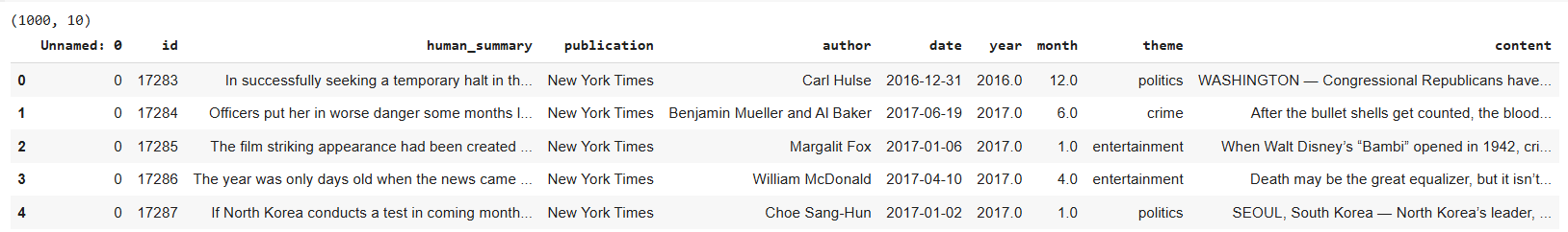
The content column contains the article content, whereas the human_summary column contains article summaries manually written by humans.
We will summarize the article content using GPT-4.1 and see how similar they are to human-generated summaries.
Several metrics exist to evaluate the text summarization performance of AI models. ROUGE metric is one such criterion.
The following script defines the calculate_rouge() function, which accepts reference and candidate summaries and calculates ROUGE scores between them.
# Function to calculate ROUGE scores
def calculate_rouge(reference, candidate):
    scorer = rouge_scorer.RougeScorer(['rouge1', 'rouge2', 'rougeL'], use_stemmer=True)
    scores = scorer.score(reference, candidate)
    return {key: value.fmeasure for key, value in scores.items()}
Next, we will define the summarize_articles_with_model() function, which accepts the LLM model ID, generates a summary of the first 20 articles in the dataset, and calculates ROUGE scores for each summary. You can summarize more than 20 articles, but for testing purposes, 20 is enough.
def summarize_articles_with_model(model_id):


    results = []
    for i, (_, row) in enumerate(dataset[:20].iterrows(), start=1):
        article = row['content']
        human_summary = row['human_summary']

        print(f"Summarizing article {i}.")

        prompt = f"Summarize the following article in 1150 characters. The summary should look like human created:\n\n{article}\n\nSummary:"

        response = client.chat.completions.create(
            model=model_id,
            messages=[{"role": "user", "content": prompt}],
            max_tokens=1150,
            temperature=0
        )
        generated_summary = response.choices[0].message.content
        rouge_scores = calculate_rouge(human_summary, generated_summary)

        results.append({
            'article_id': row.id,
            'generated_summary': generated_summary,
            'rouge1': rouge_scores['rouge1'],
            'rouge2': rouge_scores['rouge2'],
            'rougeL': rouge_scores['rougeL']
        })

    return results
In the script below we pass the gpt-4.1 model id to the summarize_articles_with_model() function and calculate mean values for ROUGE scores returned by the function.
results = summarize_articles_with_model("gpt-4.1")
results_df = pd.DataFrame(results)
mean_values = results_df[["rouge1", "rouge2", "rougeL"]].mean()
print(mean_values)
Output:
rouge1    0.332825
rouge2    0.065240
rougeL    0.150400
dtype: float64
The above output shows the ROUGE scores. These scores are pretty similar to what we achieved using the GPT-4o model in a previous article.
Multi-Class Zero-Shot Text Classification with GPT-4.1
Next, we will perform text classification using GPT-4.1. To do so, we will find sentiments of tweets in the Twitter Airline Sentiment dataset.
The following script imports the dataset and displays its header.
## Dataset download link
## https://www.kaggle.com/datasets/crowdflower/twitter-airline-sentiment?select=Tweets.csv

dataset = pd.read_csv(r"/content/Tweets.csv")
print(dataset.shape)
dataset.head()
Output:
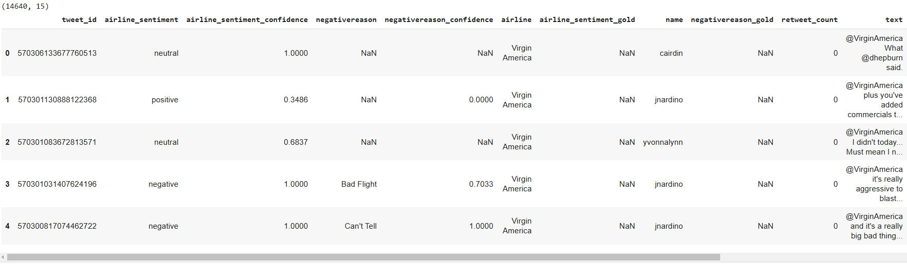
The sentiment is categorized into one of three categories: positive, negative, and neutral. We will filter 100 tweets for testing with equal distribution of the three sentiments.
# Remove rows where 'airline_sentiment' or 'text' are NaN
dataset = dataset.dropna(subset=['airline_sentiment', 'text'])

# Remove rows where 'airline_sentiment' or 'text' are empty strings
dataset = dataset[(dataset['airline_sentiment'].str.strip() != '') & (dataset['text'].str.strip() != '')]

# Filter the DataFrame for each sentiment
neutral_df = dataset[dataset['airline_sentiment'] == 'neutral']
positive_df = dataset[dataset['airline_sentiment'] == 'positive']
negative_df = dataset[dataset['airline_sentiment'] == 'negative']

# Randomly sample records from each sentiment
neutral_sample = neutral_df.sample(n=34)
positive_sample = positive_df.sample(n=33)
negative_sample = negative_df.sample(n=33)

# Concatenate the samples into one DataFrame
dataset = pd.concat([neutral_sample, positive_sample, negative_sample])

# Reset index if needed
dataset.reset_index(drop=True, inplace=True)

# print value counts
print(dataset["airline_sentiment"].value_counts())
Output:
airline_sentiment
neutral     34
positive    33
negative    33
Name: count, dtype: int64
Next, we will define the find_sentiment() function, which accepts the client and model type and predicts the sentiment for the 100 filtered tweets. The function also returns the overall accuracy for the 100 predictions.
def find_sentiment(client, model):

    tweets_list = dataset["text"].tolist()


    all_sentiments = []

    i = 0
    exceptions = 0
    while i < len(tweets_list):

        try:
            tweet = tweets_list[i]
            content = """What is the sentiment expressed in the following tweet about an airline?
            Select sentiment value from positive, negative, or neutral. Return only the sentiment value in small letters.
            tweet: {}""".format(tweet)

            sentiment_value = client.chat.completions.create(
                                  model= model,
                                  temperature = 0,
                                  max_tokens = 10,
                                  messages=[
                                        {"role": "user", "content": content}
                                    ]
                                ).choices[0].message.content

            all_sentiments.append(sentiment_value)
            i = i + 1
            print(i, sentiment_value)

        except Exception as e:
            print("===================")
            print("Exception occurred:", e)
            exceptions += 1

    print("Total exception count:", exceptions)
    accuracy = accuracy_score(all_sentiments, dataset["airline_sentiment"])
    print("Accuracy:", accuracy)
The script below calls the find_sentiment() function using the gpt-4.1 model id.
model = "gpt-4.1"
find_sentiment(client, model)
Output:
Total exception count: 0
Accuracy: 0.82
The output shows that the model achieves an accuracy of 82% for multi-class text classification task which is better than the accuracy achieved by GPT-4o in a previous article.
Multi-Label Zero-Shot Text Classification with GPT-4.1
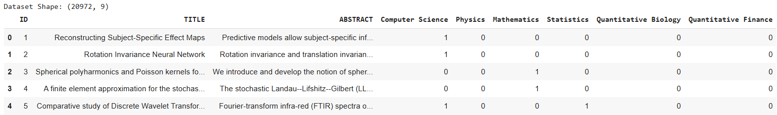
Finally, we will evaluate GPT-4.1 for a multi-label classification task using the Research Paper dataset from Kaggle.
The dataset consists of various research paper titles and abstracts and their corresponding six categories. A research paper can belong to multiple categories.
The following script imports the dataset.
## dataset download link
## https://www.kaggle.com/datasets/shivanandmn/multilabel-classification-dataset?select=train.csv

dataset = pd.read_csv(r"/content/train.csv", encoding= 'utf-8')
print(f"Dataset Shape: {dataset.shape}")
dataset.head()
Output:
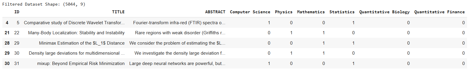
Since we are performing multi-label classification, we will only use research papers that belong to at least two categories. The following script performs this filtering.
subjects = ["Computer Science", "Physics", "Mathematics", "Statistics", "Quantitative Biology", "Quantitative Finance"]
filtered_dataset = dataset[(dataset[subjects] == 1).sum(axis=1) >= 2]
print(f"Filtered Dataset Shape: {filtered_dataset.shape}")
filtered_dataset.head()
Output:
Next, we will define the find_research_category() function, which accepts the client, LLM model ID, and dataset and performs multi-label classification.
def find_research_category(client, model, dataset):

    outputs = []
    i = 0

    for _, row in dataset.iterrows():
        title = row['TITLE']
        abstract = row['ABSTRACT']

        content = """You are an expert in various scientific domains.
                     Given the following research paper title and abstract, classify the research paper into at least two or more of the following categories:
                    - Computer Science
                    - Physics
                    - Mathematics
                    - Statistics
                    - Quantitative Biology
                    - Quantitative Finance

                    Return only a comma-separated list of the categories (e.g., [Computer Science,Physics] or [Computer Science,Physics,Mathematics]).
                    Use the exact case sensitivity and spelling of the categories provided above.

                    text: Title: {}\nAbstract: {}""".format(title, abstract)


        research_category = client.chat.completions.create(
                                model= model,
                                temperature = 0,
                                max_tokens = 100,
                                messages=[
                                      {"role": "user", "content": content}
                                  ]
                              ).choices[0].message.content


        outputs.append(research_category)
        print(i + 1, research_category)
        i += 1

    return outputs
Since the LLM model outputs are in string format, we define a function that converts them into binary numbers using the parse_outputs_to_dataframe() function below.
def parse_outputs_to_dataframe(outputs):

    subjects = ["Computer Science", "Physics", "Mathematics", "Statistics", "Quantitative Biology", "Quantitative Finance"]
    # Remove square brackets and split the subjects for each entry in outputs
    parsed_data = [item.strip('[]').split(',') for item in outputs]

    # Create an empty DataFrame with columns for each subject, initializing with 0s
    df = pd.DataFrame(0, index=range(len(parsed_data)), columns=subjects)

    # Populate the DataFrame with 1s based on the presence of each subject in each row
    for i, subjects_list in enumerate(parsed_data):
        for subject in subjects_list:
            if subject in subjects:
                df.loc[i, subject] = 1

    return df

sampled_df = filtered_dataset.sample(n=100, random_state=42)
Finally, we call the find_research_category() to predict multiple labels for the records in our dataset and then convert the output into binary labels using the parse_outputs_to_dataframe() function.
Next, we calculate hamming loss and accuracy, two commonly used criteria for multiclassification problems, to evaluate our model's performance.
model = "gpt-4.1"
outputs = find_research_category(client,
                                 model,
                                 sampled_df)

predictions = parse_outputs_to_dataframe(outputs)
targets = sampled_df[subjects]

# Calculate Hamming Loss
hamming = hamming_loss(targets, predictions)
print(f"Hamming Loss: {hamming}")

# Calculate Subset Accuracy (Exact Match Ratio)
subset_accuracy = accuracy_score(targets, predictions)
print(f"Subset Accuracy: {subset_accuracy}")
Output:
Hamming Loss: 0.18
Subset Accuracy: 0.28
The output shows that the GPT-4.1 achieves a hamming loss of 0.18 while a subset accuracy of 28%, which is less than the performance achieved by GPT-4o model in a previous article.
Conclusion
Overall, I find GPT-4.1 at par with the GPT-4o model for simpler tasks such as text classification and performance. However, GPT-4.1 is cheaper compared to GPT-4o, so I recommend using it over GPT-4o.